n-Trailer Vehicle | Alejandro Bravo-Doddoli

This page presents the dynamics of an articulated n-trailer vehicle, including mathematical results and numerical simulations.

The n-Trailer Problem

The articulated $n$-trailer vehicle has attracted considerable interest in several areas of mathematics, particularly nonholonomic mechanics, differential topology, and algebraic geometry. From the perspective of differential topology, the system is closely related to the theory of Goursat distributions, while its connections with algebraic geometry can be explored through the Monster Tower construction.

The geometric properties of the $n$-trailer system have been studied extensively. For the differential-topological approach, see:

Geometric Approach to Goursat Flags
The Car with N Trailers: Characterization of the Singular Configurations, by Frédéric Jean.

From the perspective of algebraic geometry and the Monster Tower construction, see:

Points and Curves in the Monster Tower, by Richard Montgomery and Michail Zhitomirskii.
Aspects of the Monster Tower Construction: Geometric, Combinatorial, Mechanical, Enumerative, by Susan Colley and Gary Kennedy.

Nonholonomic Dynamics

In joint work with Luis C. García-Naranjo, I studied the dynamics of an articulated $n$-trailer vehicle moving under its own inertia.

Unlike the kinematic problem, where the motion of the leading vehicle is prescribed, we study the free dynamics of the articulated n-trailer system, governed by its kinetic energy and nonholonomic constraints.

We derived the reduced equations of motion, studied their qualitative behavior, and investigated the role of conserved quantities and invariant manifolds.

Our results appear in The Dynamics of an Articulated n-Trailer Vehicle, published in Regular and Chaotic Dynamics (2015).

Connections with Optimal Control

The $n$-trailer system is also related to problems in geometric control theory.

For the case of a mobile robot with one trailer, Andrei Ardentov and P. Mashtakov developed an approach based on nilpotent approximation to study the corresponding optimal control problem.

See Control of a Mobile Robot with a Trailer Based on Nilpotent Approximation.

These complementary perspectives illustrate the connections between differential geometry, dynamical systems, and optimal control in the study of articulated vehicles.

Mathematical Model

The mechanical system depends on two geometric parameters:

$a$ is the signed distance between the center of mass of the leading vehicle and its axle, measured along the vehicle’s longitudinal axis.
$\ell$ is the distance between the contact points of two consecutive vehicles.

We assume that the center of mass of each trailer coincides with its contact point.

The parameter $a$ plays an important role in the dynamics. In particular, the qualitative behavior of the system changes significantly depending on whether $a=0$ or $a\neq 0$.

Configuration Space

The configuration of the articulated $n$-trailer vehicle is described by the position $(x,y)$ and orientation $\theta$ of the leading car, together with the relative angles $\alpha_1,\ldots,\alpha_n$ between consecutive vehicles.

The configuration space is

\[Q = SE(2)\times\mathbb T^n,\]

where $\mathbb T^n$ denotes the $n$-dimensional torus.

The nonholonomic constraints define a rank-two distribution

\[\mathcal D\subset TQ.\]

The distribution is invariant under the natural action of $SE(2)$ on the configuration space.

Nonholonomic Distribution

The nonholonomic distribution $\mathcal D$ is spanned by two $SE(2)$-invariant vector fields:

\[\begin{aligned} Z_1 &= \cos\theta\frac{\partial}{\partial x} +\sin\theta\frac{\partial}{\partial y}\\ &\quad+ \sum_{k=1}^{n}\frac{1}{\ell} \left(\prod_{j=1}^{k-2}\cos\alpha_j\right) \left( \sin\alpha_{k-1} -\cos\alpha_{k-1}\sin\alpha_k \right) \frac{\partial}{\partial\alpha_k}, \\[8pt] Z_2 &= \frac{\partial}{\partial\theta} +\frac{\partial}{\partial\alpha_1}. \end{aligned}\]

We use the conventions $\alpha_0=0$ and that a product over an empty index range equals $1$.

These vector fields define the quasi-velocities:

\[\begin{aligned} u &= \text{speed of the leading car along its axis},\\ \omega &= \text{angular velocity of the leading car}. \end{aligned}\]

Symmetry Reduction

Since both the kinetic energy and the nonholonomic distribution are invariant under the natural action of (SE(2)), we can exploit this symmetry to obtain reduced equations of motion.

The reduced phase space is

\[\mathcal D/SE(2)\cong\mathbb R^2\times\mathbb T^n,\]

with coordinates

\[(u,\omega,\alpha_1,\ldots,\alpha_n).\]

Reduced Equations of Motion

The dynamics of the articulated n-trailer vehicle can be described by a system of $n+2$ nonlinear ordinary differential equations.

Theorem 1. The reduced equations of motion are

\[\begin{aligned} \dot{u} &= -\frac{1}{2R(\alpha)} \left( \sum_{k=1}^{n} A_k\frac{\partial R}{\partial\alpha_k} \right)u^2 +\frac{Q(\alpha)}{\ell^2R(\alpha)}u\omega +\frac{Ma}{R(\alpha)}\omega^2, \\[8pt] \dot{\omega} &= -\frac{Ma}{J_0+Ma^2}u\omega, \\[8pt] \dot{\alpha}_1 &= \omega-\frac{u}{\ell}\sin\alpha_1, \\[8pt] \dot{\alpha}_k &= \frac{u}{\ell} \left( \prod_{j=1}^{k-2}\cos\alpha_j \right) \left( \sin\alpha_{k-1} -\cos\alpha_{k-1}\sin\alpha_k \right), \quad k=2,\ldots,n. \end{aligned}\]

Here,

\[A_k= \frac{1}{\ell} \left( \prod_{j=1}^{k-2}\cos\alpha_j \right) \left( \sin\alpha_{k-1} -\cos\alpha_{k-1}\sin\alpha_k \right), \qquad k=1,\ldots,n.\]

We use the conventions $\alpha_0=0$ and that a product over an empty index range equals $1$.

The functions $Q(\alpha)$ and $R(\alpha)$ are defined by

\[\begin{aligned} Q(\alpha) &= \cos\alpha_1\sin\alpha_1 \left[ m\ell^2 \sum_{j=1}^{n} \left( \prod_{k=2}^{j}\cos^2\alpha_k \right) - J\prod_{k=2}^{n}\cos^2\alpha_k \right], \\[12pt] R(\alpha) &= M + m\left( \sum_{j=1}^{n} \prod_{k=1}^{j}\cos^2\alpha_k \right) + \frac{J}{\ell^2} \left( 1-\prod_{k=1}^{n}\cos^2\alpha_k \right). \end{aligned}\]

Conservation of Energy

The articulated $n$-trailer vehicle is a nonholonomic mechanical system whose motion conserves kinetic energy.

The reduced energy is given by

\[E(\alpha,u,\omega) = \frac{1}{2} \left[ R(\alpha)u^2 + (J_0+Ma^2)\omega^2 \right].\]

Along every solution of the reduced equations of motion,

\[\frac{dE}{dt}=0.\]

Since the kinetic energy defines a positive-definite quadratic form in the quasi-velocities ((u,\omega)), every positive energy level is diffeomorphic to an ((n+1))-dimensional torus:

\[E^{-1}(E_0)\cong\mathbb T^{n+1}, \qquad E_0>0.\]

Qualitative Dynamics

The qualitative behavior of the articulated $n$-trailer vehicle depends on the parameter $a$, which describes the position of the center of mass of the leading vehicle relative to its axle.

We distinguish two cases: $a\neq 0$ and $a=0$.

Dynamics for $a=0$

When $a=0$, the angular velocity $\omega$ is an additional first integral of the reduced equations of motion

Fixing the energy and angular velocity restricts the dynamics to invariant $n$-dimensional tori.

For $n=2$, the dynamics on these tori can be visualized through phase portraits.

Phase Portraits for $n=2$

For two trailers, the dynamics on the invariant two-dimensional tori exhibit different qualitative behaviors depending on the energy.

The following phase portraits illustrate the bifurcations of the reduced dynamics as the energy varies.

Regime I: $0<E<E_c^{(1)}$

In this energy range, the phase portrait suggests that the reduced dynamics have no equilibrium points or periodic orbits.

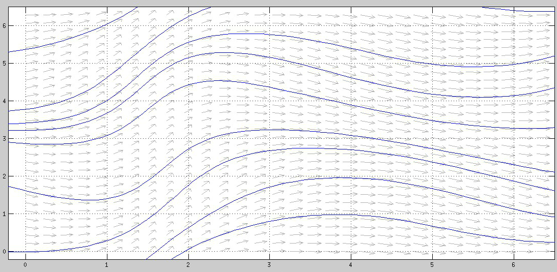
Phase portrait of the n-trailer dynamics below the first critical energy

Phase portrait for the energy range $0<E<E_c^{(1)}$.

Numerical simulation

Motion of the articulated two-trailer vehicle for $0<E<E_c^{(1)}$.

Regime II: $E=E_c^{(1)}$

At the first critical energy, the reduced dynamics exhibit a nonhyperbolic periodic orbit with a center manifold. The periodic orbit is stable from the left and unstable from the right.

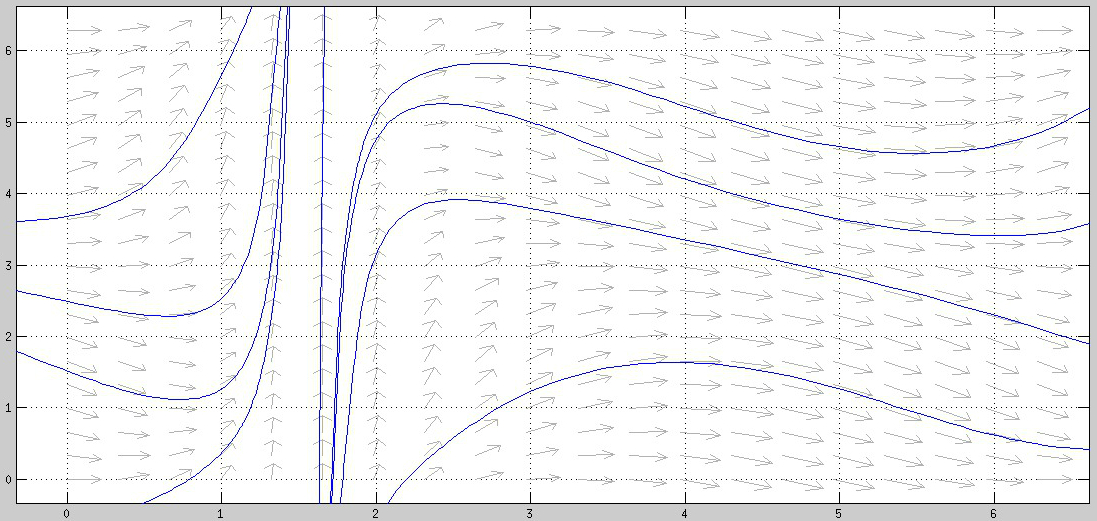
Phase portrait at the first critical energy $E=E_c^{(1)}$.

Numerical simulation

Motion of the articulated two-trailer vehicle at the first critical energy $E=E_c^{(1)}$.

Regime III: $E_c^{(1)}<E<E_c^{(2)}$

Between the two critical energy values, the reduced dynamics exhibit two periodic orbits.

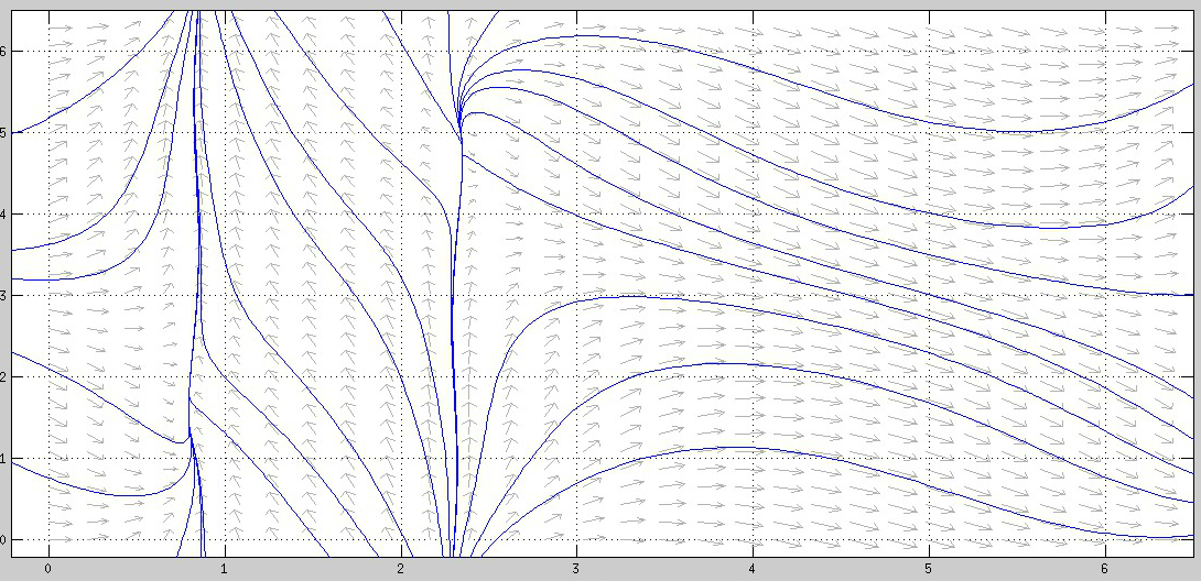
Phase portrait between the two critical energy values

Phase portrait for $E_c^{(1)}<E<E_c^{(2)}$.

Numerical simulation

Motion of the articulated two-trailer vehicle for $E_c^{(1)}<E<E_c^{(2)}$.

Regime IV: $E=E_c^{(2)}$

At the second critical energy, the reduced dynamics have two degenerate equilibrium points corresponding to saddle-node bifurcations.

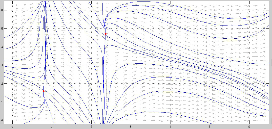
Phase portrait at the second critical energy $E=E_c^{(2)}$.

Numerical simulation

Motion of the articulated two-trailer vehicle at the second critical energy $E=E_c^{(2)}$.

Regime V: $E>E_c^{(2)}$

Above the second critical energy, the reduced dynamics have four equilibrium points: two saddles and two nodes.

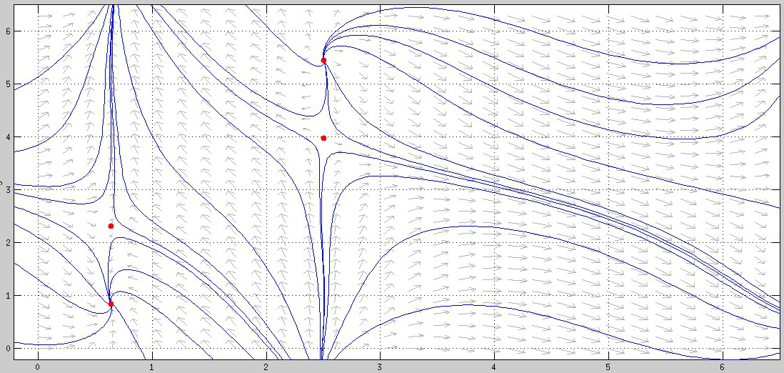
Phase portrait above the second critical energy

Phase portrait for $E>E_c^{(2)}$.

Numerical simulation

Motion of the articulated two-trailer vehicle for $E>E_c^{(2)}$.